Urban Density for bike?

Hello,
I’m using a self-hosted GraphHopper instance for a bike route planner, which can generate random routes with the round_trip option.

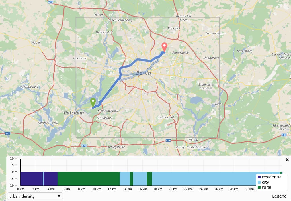
I would like to include the urban_density in the details of the generated routes AND also use urban_density in my custom_model request to prioritize roads outside cities)

urban_density is empty on the generated routes.
Here my config:

graphhopper:

# OpenStreetMap input file PBF or XML, can be changed via command line -Ddw.graphhopper.datareader.file=some.pbf

datareader.file: “”

# Local folder used by graphhopper to store its data

graph.location: /data/default-gh/

##### Routing Profiles ####

# Routing can be done only for profiles listed below. For more information about profiles and custom profiles have a

# look into the documentation at docs/core/profiles.md or the examples under web/src/test/java/com/graphhopper/application/resources/

# or the CustomWeighting class for the raw details.

#

# In general a profile consists of the following

# - name (required): a unique string identifier for the profile

# - vehicle (required): refers to the `graph.vehicles` used for this profile

# - weighting (required): the weighting used for this profile like custom,fastest,shortest or short_fastest

# - turn_costs (true/false, default: false): whether or not turn restrictions should be applied for this profile.

#

# Depending on the above fields there are other properties that can be used, e.g.

# - distance_factor: 0.1 (can be used to fine tune the time/distance trade-off of short_fastest weighting)

# - u_turn_costs: 60 (time-penalty for doing a u-turn in seconds (only possible when `turn_costs: true`)).

# Note that since the u-turn costs are given in seconds the weighting you use should also calculate the weight

# in seconds, so for example it does not work with shortest weighting.

# - custom_model_file: when you specified “weighting: custom” you need to set a json file inside your custom_model_folder

# or working directory that defines the custom_model. If you want an empty model you can also set “custom_model_file: empty”.

# You can also use th e`custom_model` field instead and specify your custom model in the profile directly.

#

# To prevent long running routing queries you should usually enable either speed or hybrid mode for all the given

# profiles (see below). Or at least limit the number of `routing.max_visited_nodes`.

profiles:

- name: mtb

custom_model_files: [mtb.json, bike_elevation.json]

- name: bike

custom_model_files: [bike.json, bike_elevation.json]

- name: racingbike

custom_model_files: [racingbike.json, bike_elevation.json]

#

# - name: mtb

# custom_model_files: [mtb.json, bike_elevation.json]

# Speed mode:

# Its possible to speed up routing by doing a special graph preparation (Contraction Hierarchies, CH). This requires

# more RAM/disk space for holding the prepared graph but also means less memory usage per request. Using the following

# list you can define for which of the above routing profiles such preparation shall be performed. Note that to support

# profiles with `turn_costs: true` a more elaborate preparation is required (longer preparation time and more memory

# usage) and the routing will also be slower than with `turn_costs: false`.

profiles_ch:

# Hybrid mode:

# Similar to speed mode, the hybrid mode (Landmarks, LM) also speeds up routing by doing calculating auxiliary data

# in advance. Its not as fast as speed mode, but more flexible.

#

# Advanced usage: It is possible to use the same preparation for multiple profiles which saves memory and preparation

# time. To do this use e.g. `preparation_profile: my_other_profile` where `my_other_profile` is the name of another

# profile for which an LM profile exists. Important: This only will give correct routing results if the weights

# calculated for the profile are equal or larger (for every edge) than those calculated for the profile that was used

# for the preparation (`my_other_profile`)

profiles_lm:

#### Encoded Values ####

# Add additional information to every edge. Used for path details (#1548*) and custom models (docs/core/custom-models.md)*

# Default values are: road_class,road_class_link,road_environment,max_speed,road_access

# More are: surface,smoothness,max_width,max_height,max_weight,hgv,max_axle_load,max_length,hazmat,hazmat_tunnel,hazmat_water,toll,track_type,

# mtb_rating, hike_rating,horse_rating,lanes

# GH 11:

graph.encoded_values: bike_priority, mtb_rating, hike_rating, country, road_class, bike_access, roundabout, bike_average_speed, average_slope, mtb_priority, mtb_access, mtb_average_speed, racingbike_priority, racingbike_access, racingbike_average_speed, surface, track_type, max_slope, urban_density

#### Speed, hybrid and flexible mode ####

# To make CH preparation faster for multiple profiles you can increase the default threads if you have enough RAM.

# Change this setting only if you know what you are doing and if the default worked for you.

# prepare.ch.threads: 1

# To tune the performance vs. memory usage for the hybrid mode use

# prepare.lm.landmarks: 16

# Make landmark preparation parallel if you have enough RAM. Change this only if you know what you are doing and if

# the default worked for you.

# prepare.lm.threads: 1

#### Elevation ####

# To populate your graph with elevation data use SRTM, default is noop (no elevation). Read more about it in docs/core/elevation.md

graph.elevation.provider: srtm

# default location for cache is /tmp/srtm

graph.elevation.cache_dir: /usr/src/app/elevation/

# If you have a slow disk or plenty of RAM change the default MMAP to:

graph.elevation.dataaccess: MMAP_STORE

# To enable bilinear interpolation when sampling elevation at points (default uses nearest neighbor):

# graph.elevation.interpolate: bilinear

# Reduce ascend/descend per edge without changing the maximum slope:

# graph.elevation.edge_smoothing: ramer

# removes elevation fluctuations up to max_elevation (in meter) and replaces the elevation with a value based on the average slope

# graph.elevation.edge_smoothing.ramer.max_elevation: 5

# A potentially bigger reduction of ascend/descend is possible, but maximum slope will often increase (do not use when average_slope or maximum_slope shall be used in a custom_model)

# graph.elevation.edge_smoothing: moving_average

# To increase elevation profile resolution, use the following two parameters to tune the extra resolution you need

# against the additional storage space used for edge geometries. You should enable bilinear interpolation when using

# these features (see #1953 for details).

# - first, set the distance (in meters) at which elevation samples should be taken on long edges

# graph.elevation.long_edge_sampling_distance: 60

# - second, set the elevation tolerance (in meters) to use when simplifying polylines since the default ignores

# elevation and will remove the extra points that long edge sampling added

# graph.elevation.way_point_max_distance: 10

#### Urban density (built-up areas) ####

# This feature allows classifying roads into ‘rural’, ‘residential’ and ‘city’ areas (encoded value ‘urban_density’)

# Use 1 or more threads to enable the feature

# graph.urban_density.threads: 8

# Use higher/lower sensitivities if too little/many roads fall into the according categories.

# Using smaller radii will speed up the classification, but only change these values if you know what you are doing.

# If you do not need the (rather slow) city classification set city_radius to zero.

graph.urban_density.residential_radius: 300

graph.urban_density.residential_sensitivity: 60

graph.urban_density.city_radius: 2000

graph.urban_density.city_sensitivity: 30

#### Subnetworks ####

# In many cases the road network consists of independent components without any routes going in between. In

# the most simple case you can imagine an island without a bridge or ferry connection. The following parameter

# allows setting a minimum size (number of edges) for such detached components. This can be used to reduce the number

# of cases where a connection between locations might not be found.

prepare.min_network_size: 200

prepare.subnetworks.threads: 1

#### Routing ####

# You can define the maximum visited nodes when routing. This may result in not found connections if there is no

# connection between two points within the given visited nodes. The default is Integer.MAX_VALUE. Useful for flexibility mode

# routing.max_visited_nodes: 1000000

# Control how many active landmarks are picked per default, this can improve query performance

# routing.lm.active_landmarks: 4

# You can limit the max distance between two consecutive waypoints of flexible routing requests to be less or equal

# the given distance in meter. Default is set to 1000km.

routing.non_ch.max_waypoint_distance: 1000000

#### Storage ####

import.osm.ignored_highways:

# configure the memory access, use RAM_STORE for well equipped servers (default and recommended)

graph.dataaccess.default_type: MMAP_STORE

# will write way names in the preferred language (language code as defined in ISO 639-1 or ISO 639-2):

# datareader.preferred_language: en

# Sort the graph after import to make requests roughly ~10% faster. Note that this requires significantly more RAM on import.

# graph.do_sort: true

#### Custom Areas ####

# GraphHopper reads GeoJSON polygon files including their properties from this directory and makes them available

# to all tag parsers and vehicles. Country borders (see countries.geojson) are always included automatically.

# custom_areas.directory: path/to/custom_areas

#### Country Rules ####

# GraphHopper applies country-specific routing rules during import (not enabled by default).

# You need to redo the import for changes to take effect.

# country_rules.enabled: true

# Dropwizard server configuration

server:

application_connectors:

- type: http

port: 8989

# for security reasons bind to localhost

bind_host: localhost

request_log:

appenders:

admin_connectors:

- type: http

port: 8990

bind_host: localhost

# See Dropwizard Core — Dropwizard

logging:

appenders:

- type: file

time_zone: UTC

current_log_filename: logs/graphhopper.log

log_format: “%d{yyyy-MM-dd HH:mm:ss.SSS} [%thread] %-5level %logger{36} - %msg%n”

archive: true

archived_log_filename_pattern: ./logs/graphhopper-%d.log.gz

archived_file_count: 7

never_block: true

- type: console

time_zone: UTC

threshold: WARN

log_format: “%d{yyyy-MM-dd HH:mm:ss.SSS} [%thread] %-5level %logger{36} - %msg%n”

(I’m using MMAP_STORE because I miss more RAM)

Thanks :slight_smile:

You need to enable filling the encoded value via setting this to at least 1. (interesting that you were able to use it without an error was thrown. We should improve this)

My mistake,
During my test I had indeed uncommented “graph.urban_density.threads: 1” (otherwise I do get an error during import).

To be more precise, on my local instance, regardless of the route (even if I go through a large city), I always get with bike profile:

“urban_density”: [
[0, 399, “rural”],
[399, 680, “rural”]
]

Whereas for the same route on your public instance (but using the “car” profile), I can see that it works correctly:

{
“priority”: [
{
“if”: “urban_density==RURAL”,
“multiply_by”: “1”
},
{
“if”: “urban_density==RESIDENTIAL”,
“multiply_by”: “1”
},
{
“if”: “urban_density==CITY”,
“multiply_by”: “0.1”
}
]
}

Urban density with car profile

Link seem broken with the editor, so here the queryString: ?point=50.741257%2C4.470005&point=50.842372%2C4.366863&point=50.914528%2C4.29388&profile=car&layer=OpenStreetMap&custom_model=%7B%22priority%22%3A%5B%7B%22if%22%3A%22urban_density%3D%3DRURAL%22%2C%22multiply_by%22%3A%221%22%7D%2C%7B%22if%22%3A%22urban_density%3D%3DRESIDENTIAL%22%2C%22multiply_by%22%3A%221%22%7D%2C%7B%22if%22%3A%22urban_density%3D%3DCITY%22%2C%22multiply_by%22%3A%220.1%22%7D%5D%7D

@karussell sorry to bother you, do you have an idea why I always have “rural” ?

When you remove the graph-cache and try to do the import again, do you see something like:

...UrbanDensityCalculator - Calculating residential areas …, radius=400.0, sensitivity=6000.0, threads=8
...UrbanDensityCalculator - Finished calculating residential areas, took: 15.066945s
...UrbanDensityCalculator - Calculating city areas ..., radius=1500.0, sensitivity=1000.0, threads=8
...UrbanDensityCalculator - Finished calculating city areas, took: 171.99081s

in the logs? If no, then the config is still wrong. ( The city areas calculation always takes a bit long, but you can disable it or throw more threads to it :slight_smile: )

You should then also be able to use the /route endpoint and see the urban_density details.

If you want to see the urban density in GraphHopper Maps then this is currently not possible in the bundled maps and instead you install GraphHopper Maps from source and add urban_density to the request details in your config-local.js:

request: {
  details: ["road_class","road_environment","road_access","max_speed","average_speed","country", "urban_density"],
}

I just tried it out for berlin-latest.osm.pbf:

note, your statements that use "multiply_by":"1" are not necessary as the default is already 1.

@karussell Thanks, yes I have :

2025-09-16 15:55:12.142 [main] INFO c.g.r.util.UrbanDensityCalculator - Calculating residential areas …, radius=300.0, sensitivity=60.0, threads=1
2025-09-16 15:56:10.026 [main] INFO c.g.r.util.UrbanDensityCalculator - Finished calculating residential areas, took: 57.8828s
2025-09-16 15:56:10.026 [main] INFO c.g.r.util.UrbanDensityCalculator - Calculating city areas …, radius=2000.0, sensitivity=30.0, threads=1
2025-09-16 15:56:11.782 [main] INFO c.g.r.util.UrbanDensityCalculator - Finished calculating city areas, took: 1.7556648s

AND :

graphhopper:

# OpenStreetMap input file PBF or XML, can be changed via command line -Ddw.graphhopper.datareader.file=some.pbf

datareader.file: “”

# Local folder used by graphhopper to store its data

graph.location: /data/default-gh/

##### Routing Profiles ####

# Routing can be done only for profiles listed below. For more information about profiles and custom profiles have a

# look into the documentation at docs/core/profiles.md or the examples under web/src/test/java/com/graphhopper/application/resources/

# or the CustomWeighting class for the raw details.

#

# In general a profile consists of the following

# - name (required): a unique string identifier for the profile

# - vehicle (required): refers to the `graph.vehicles` used for this profile

# - weighting (required): the weighting used for this profile like custom,fastest,shortest or short_fastest

# - turn_costs (true/false, default: false): whether or not turn restrictions should be applied for this profile.

#

# Depending on the above fields there are other properties that can be used, e.g.

# - distance_factor: 0.1 (can be used to fine tune the time/distance trade-off of short_fastest weighting)

# - u_turn_costs: 60 (time-penalty for doing a u-turn in seconds (only possible when `turn_costs: true`)).

# Note that since the u-turn costs are given in seconds the weighting you use should also calculate the weight

# in seconds, so for example it does not work with shortest weighting.

# - custom_model_file: when you specified “weighting: custom” you need to set a json file inside your custom_model_folder

# or working directory that defines the custom_model. If you want an empty model you can also set “custom_model_file: empty”.

# You can also use th e`custom_model` field instead and specify your custom model in the profile directly.

#

# To prevent long running routing queries you should usually enable either speed or hybrid mode for all the given

# profiles (see below). Or at least limit the number of `routing.max_visited_nodes`.

profiles:

- name: mtb

custom_model_files: [mtb.json, bike_elevation.json]

- name: bike

custom_model_files: [bike.json, bike_elevation.json]

- name: racingbike

custom_model_files: [racingbike.json, bike_elevation.json]

#

# - name: mtb

# custom_model_files: [mtb.json, bike_elevation.json]

# Speed mode:

# Its possible to speed up routing by doing a special graph preparation (Contraction Hierarchies, CH). This requires

# more RAM/disk space for holding the prepared graph but also means less memory usage per request. Using the following

# list you can define for which of the above routing profiles such preparation shall be performed. Note that to support

# profiles with `turn_costs: true` a more elaborate preparation is required (longer preparation time and more memory

# usage) and the routing will also be slower than with `turn_costs: false`.

profiles_ch:

# Hybrid mode:

# Similar to speed mode, the hybrid mode (Landmarks, LM) also speeds up routing by doing calculating auxiliary data

# in advance. Its not as fast as speed mode, but more flexible.

#

# Advanced usage: It is possible to use the same preparation for multiple profiles which saves memory and preparation

# time. To do this use e.g. `preparation_profile: my_other_profile` where `my_other_profile` is the name of another

# profile for which an LM profile exists. Important: This only will give correct routing results if the weights

# calculated for the profile are equal or larger (for every edge) than those calculated for the profile that was used

# for the preparation (`my_other_profile`)

profiles_lm:

#### Encoded Values ####

# Add additional information to every edge. Used for path details (#1548*) and custom models (docs/core/custom-models.md)*

# Default values are: road_class,road_class_link,road_environment,max_speed,road_access

# More are: surface,smoothness,max_width,max_height,max_weight,hgv,max_axle_load,max_length,hazmat,hazmat_tunnel,hazmat_water,toll,track_type,

# mtb_rating, hike_rating,horse_rating,lanes

# GH 11:

graph.encoded_values: bike_priority, mtb_rating, hike_rating, country, road_class, bike_access, roundabout, bike_average_speed, average_slope, mtb_priority, mtb_access, mtb_average_speed, racingbike_priority, racingbike_access, racingbike_average_speed, surface, track_type, max_slope, urban_density

#### Speed, hybrid and flexible mode ####

# To make CH preparation faster for multiple profiles you can increase the default threads if you have enough RAM.

# Change this setting only if you know what you are doing and if the default worked for you.

# prepare.ch.threads: 1

# To tune the performance vs. memory usage for the hybrid mode use

# prepare.lm.landmarks: 16

# Make landmark preparation parallel if you have enough RAM. Change this only if you know what you are doing and if

# the default worked for you.

# prepare.lm.threads: 1

#### Elevation ####

# To populate your graph with elevation data use SRTM, default is noop (no elevation). Read more about it in docs/core/elevation.md

graph.elevation.provider: srtm

# default location for cache is /tmp/srtm

graph.elevation.cache_dir: /usr/src/app/elevation/

# If you have a slow disk or plenty of RAM change the default MMAP to:

graph.elevation.dataaccess: MMAP_STORE

# To enable bilinear interpolation when sampling elevation at points (default uses nearest neighbor):

# graph.elevation.interpolate: bilinear

# Reduce ascend/descend per edge without changing the maximum slope:

# graph.elevation.edge_smoothing: ramer

# removes elevation fluctuations up to max_elevation (in meter) and replaces the elevation with a value based on the average slope

# graph.elevation.edge_smoothing.ramer.max_elevation: 5

# A potentially bigger reduction of ascend/descend is possible, but maximum slope will often increase (do not use when average_slope or maximum_slope shall be used in a custom_model)

# graph.elevation.edge_smoothing: moving_average

# To increase elevation profile resolution, use the following two parameters to tune the extra resolution you need

# against the additional storage space used for edge geometries. You should enable bilinear interpolation when using

# these features (see #1953 for details).

# - first, set the distance (in meters) at which elevation samples should be taken on long edges

# graph.elevation.long_edge_sampling_distance: 60

# - second, set the elevation tolerance (in meters) to use when simplifying polylines since the default ignores

# elevation and will remove the extra points that long edge sampling added

# graph.elevation.way_point_max_distance: 10

#### Urban density (built-up areas) ####

# This feature allows classifying roads into ‘rural’, ‘residential’ and ‘city’ areas (encoded value ‘urban_density’)

# Use 1 or more threads to enable the feature

graph.urban_density.threads: 1

# Use higher/lower sensitivities if too little/many roads fall into the according categories.

# Using smaller radii will speed up the classification, but only change these values if you know what you are doing.

# If you do not need the (rather slow) city classification set city_radius to zero.

graph.urban_density.residential_radius: 300

graph.urban_density.residential_sensitivity: 60

graph.urban_density.city_radius: 2000

graph.urban_density.city_sensitivity: 30

#### Subnetworks ####

# In many cases the road network consists of independent components without any routes going in between. In

# the most simple case you can imagine an island without a bridge or ferry connection. The following parameter

# allows setting a minimum size (number of edges) for such detached components. This can be used to reduce the number

# of cases where a connection between locations might not be found.

prepare.min_network_size: 200

prepare.subnetworks.threads: 1

#### Routing ####

# You can define the maximum visited nodes when routing. This may result in not found connections if there is no

# connection between two points within the given visited nodes. The default is Integer.MAX_VALUE. Useful for flexibility mode

# routing.max_visited_nodes: 1000000

# Control how many active landmarks are picked per default, this can improve query performance

# routing.lm.active_landmarks: 4

# You can limit the max distance between two consecutive waypoints of flexible routing requests to be less or equal

# the given distance in meter. Default is set to 1000km.

routing.non_ch.max_waypoint_distance: 1000000

#### Storage ####

import.osm.ignored_highways:

# configure the memory access, use RAM_STORE for well equipped servers (default and recommended)

graph.dataaccess.default_type: MMAP_STORE

# will write way names in the preferred language (language code as defined in ISO 639-1 or ISO 639-2):

# datareader.preferred_language: en

# Sort the graph after import to make requests roughly ~10% faster. Note that this requires significantly more RAM on import.

# graph.do_sort: true

#### Custom Areas ####

# GraphHopper reads GeoJSON polygon files including their properties from this directory and makes them available

# to all tag parsers and vehicles. Country borders (see countries.geojson) are always included automatically.

# custom_areas.directory: path/to/custom_areas

#### Country Rules ####

# GraphHopper applies country-specific routing rules during import (not enabled by default).

# You need to redo the import for changes to take effect.

# country_rules.enabled: true

# Dropwizard server configuration

server:

application_connectors:

- type: http

port: 8989

# for security reasons bind to localhost

bind_host: localhost

request_log:

appenders:

admin_connectors:

- type: http

port: 8990

bind_host: localhost

# See Dropwizard Core — Dropwizard

logging:

level: DEBUG # ou DEBUG si tu veux du très verbeux

appenders:

- type: file

time_zone: UTC

current_log_filename: logs/graphhopper.log

log_format: “%d{yyyy-MM-dd HH:mm:ss.SSS} [%thread] %-5level %logger{36} - %msg%n”

archive: true

archived_log_filename_pattern: ./logs/graphhopper-%d.log.gz

archived_file_count: 7

never_block: true

- type: console

time_zone: UTC

threshold: DEBUG

log_format: “%d{yyyy-MM-dd HH:mm:ss.SSS} [%thread] %-5level %logger{36} - %msg%n”

in /route body:

{
“points”: [
[
13.121851160949193,
52.3856331307951
],
[
13.516072716124986,
52.588894111315
]
],
“profile”: “racingbike”,
“elevation”: true,
“instructions”: true,
“locale”: “fr_FR”,
“points_encoded”: true,
“points_encoded_multiplier”: 1000000,
“details”: [
“road_class”,
“road_environment”,
“max_speed”,
“average_speed”,
“urban_density”
],
“snap_preventions”: [
“ferry”
],
“alternative_route.max_paths”: 3,
“algorithm”: “alternative_route”
}

AND result always “rural” in the details response:

“urban_density”: [
[
0,
798,
“rural”
]
],

Why not use the recommended config values?

Later you can always tune it (if you know what they mean :slight_smile: )

Because I’m a noob :slight_smile:

I’m using Docker Compose and I naïvely took the config from here without thinking too much about it:
https://github.com/IsraelHikingMap/Site/blob/main/gh-config.yml

Thanks, it’s working now.

And by the way, thank you for all the work you (and your colleagues) are doing on GraphHopper, it’s really an amazing and powerful product :slight_smile:

here without thinking too much about it:

Ah, ok, thanks for pointing this out. Feel free to raise an issue there as these might be the default values for some previous version or maybe these values work for them (?) … they’ll know :slight_smile:

Thanks, it’s working now.

:+1:

And by the way, thank you for all the work you (and your colleagues) are doing on GraphHopper, it’s really an amazing and powerful product :slight_smile:

Thanks for your kind words :slight_smile: